表观基因组学研究方法——ATAC-seq
date: 2023-11-16 update slug: ATAC-seq key: ATAC-seq,Bioinformatics,Epigenetics ref: https://informatics.fas.harvard.edu/atac-seq-guidelines cover:
by 赵华男

ATAC-seq (Assay for Transposase-Accessible Chromatin with high-throughput sequencing)
- peak calling
- peak independent / dependent quality metrics
-
differential accessibility analysis
-
ATAC-seq is a method for determining chromatin accessibility across the genome. It utilizes a hyperactive Tn5 transposase to insert sequencing adapters into open chromatin regions. High-throughput sequencing then yields reads that indicate these regions of increased accessibility. ATAC-seq是一种确定整个基因组染色质可及性的方法。它利用高活性的Tn5转座酶将测序接头插入开放的染色质区域。然后,高通量测序产生指示这些区域可访问性增加的读取。

⭐️bulk ATAC-seq
General QC
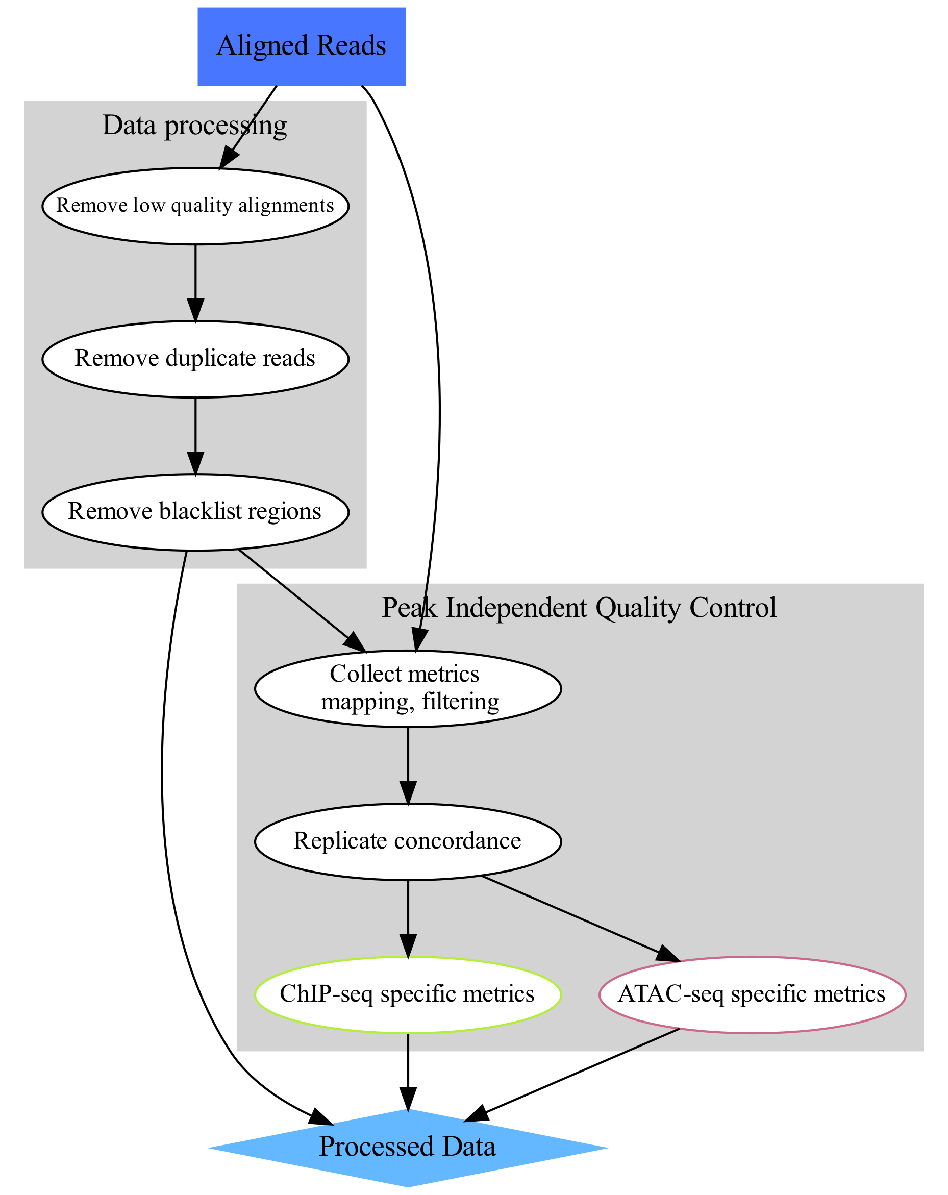
- Data processing
- Remove low quality alignments 删除低质量的对齐
- Remove duplicate reads 删除重复读取
- Remove blacklist regions 删除黑名单区域
- Peak Independent Quality Control 与peak无关的质量控制
- Collect metrics(mapping、filtering) 收集指标(mapping、filtering)
- Replicate concordance 重复间的一致性
- ChIP-seq specific metrics ChIP-seq特殊指标
- ATAC-seq specific metrics ATAC-seq特殊指标
The aim of this part is to perform general signal structure agnostic (i.e. peak - independent) quality control (lower-right part of the concept map). 这一部分的目的是执行与信号结构无关(即与peak无关)的常规质量控制(概念图的右下部分)。
These include: assessment of read coverage along the genome 评估基因组的读取覆盖率 replicate congruency 重复间的一致性
plotFingerprint
plotFingerprint \
    --bamfiles \
        ENCFF363HBZ.chr14.proc.bam \
        ENCFF398QLV.chr14.proc.bam \
        ENCFF045OAB.chr14.proc.bam \
        ENCFF828ZPN.chr14.proc.bam \
    --binSize=1000 \
    --plotFile NKcellsATAC_chr14.fingerprint.pdf \
    --labels \
        ENCFF363HBZ \
        ENCFF398QLV \
        ENCFF045OAB \
        ENCFF828ZPN \
    -p 8 \
    &> fingerprint.log
Have a look at NKcellsATAC_chr14.fingerprint.pdf, read deepTools What the plots tell you:
An ideal input with perfect uniform distribution of reads along the genome (i.e. without enrichments in open chromatin etc.) and infinite sequencing coverage should generate a straight diagonal line. 在理想情况下,如果input的reads沿着基因组均匀分布(即,没有在open chromatin富集的input),则该样本会在途中产生一条直线对角线. A very specific and strong ChIP enrichment will be indicated by a prominent and steep rise of the cumulative sum towards the highest rank. 一个非常specific和strong的 ChIP 富集将通过累积总和向最高等级的显着和急剧上升来表示。(就像图中表述的一样陡峭的上升) This means that a big chunk of reads from the ChIP sample is located in few bins which corresponds to high, narrow enrichments typically seen for transcription factors. 这意味着来自 ChIP 样品的大量reads分布于少量的bins,这对应于转录因子通常看到的peak很高且window很窄的富集模式。
and answer * does it indicate a good sample quality, i.e. signal present in narrow regions?

Replicate Clustering
To assess overall similarity between libraries from different samples one can compute sample clustering heatmaps using multiBamSummary and plotCorrelation in bins mode from deepTools. 要评估来自不同样本的库之间的整体相似性,可以使用 deepTools 的 multiBamSummary 和 plotCorrelation 在箱模式下计算样本聚类热图。
In this method the genome is divided into bins of specified size (--binSize parameter) and reads mapped to each bin are counted. The resulting signal profiles are used to cluster libraries to identify groups of similar signal profile. 在这种方法中,基因组被划分为指定大小的箱(--binSize参数),并计数映射到每个箱的读取。生成的信号配置文件用于对库进行聚类,以识别相似信号配置文件的组。
We chose to compute pairwise Spearman correlation coefficients for this step, as they are based on ranks of each bin rather than signal values. 我们选择在此步骤中计算成对的 Spearman 相关系数,因为它们基于每个箱的秩而不是信号值。
In this part we use bam files filtered previously, to save time. 在这一部分中,我们使用之前过滤的bam文件,以节省时间。
multiBamSummary bins \
    --bamfiles \
        ENCFF363HBZ.chr14.proc.bam \
        ENCFF398QLV.chr14.proc.bam \
        ENCFF045OAB.chr14.proc.bam \
        ENCFF828ZPN.chr14.proc.bam \
    --labels \
        ENCFF363HBZ \
        ENCFF398QLV \
        ENCFF045OAB \
        ENCFF828ZPN \
    --outFileName multiBamArray_NKcellsATAC_chr14.npz \
    --binSize 5000 \
    -p 8 \
    &> multiBamSummary.log

plotCorrelation \
    --corData multiBamArray_NKcellsATAC_chr14.npz \
    --plotFile NKcellsATAC_chr14_correlation_bin.pdf \
    --outFileCorMatrix NKcellsATAC_chr14_correlation_bin.txt \
    --whatToPlot heatmap \
    --corMethod spearman
You can copy the resulting file to your local system to view it.
What do you think? which samples are similar? are the clustering results as you would have expected them to be?
Correlation of binned ATAC-seq signal in NK cells.

In addition to these general procedures, several specialised assay - specific quality metrics exist, which probe signal characteristics related to each method. These are key QC metrics to evaluate the experiment and should always be colleced during the QC step. The method specific tutorials are: ATACseq and ChIPseq.除了这些一般程序之外,还存在几种专门的检测 - 特定的质量指标,这些指标探测与每种方法相关的信号特征。这些是评估实验的关键QC指标,应始终在QC步骤中收集。特定于方法的教程是:ATACseq 和 ChIPseq。
We can now follow with ATACseq specifc QC methods.我们现在可以遵循ATACseq特定的QC方法。
Specifc QC methods for ATACseq
This tutorial is a continuation of General QC
The aim of this part of the data analysis workflow is to collect ATAC-seq specific quality metrics: fragment length distribution; presence of signal in nuclesome-free regions (NFR) and mononucleosome fractions; * enrichment of signal in transcription start site (TSS) regions.
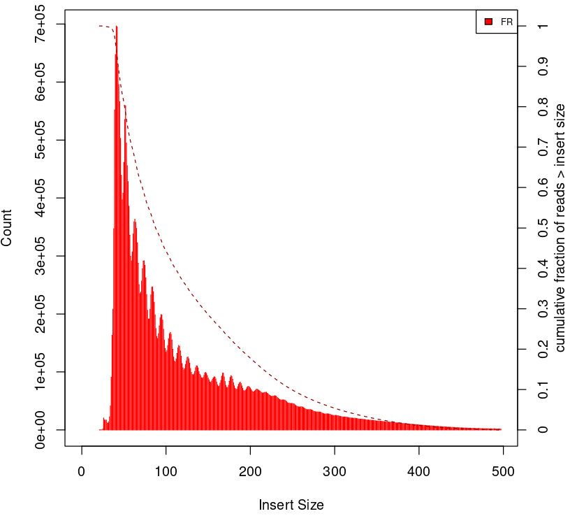
Fragment Length Distribution
In ATAC-seq experiments, tagmentation of Tn5 transposases produces signature size pattern of fragments derived from nucleosome-free regions (NFR), mononucleosome, dinucleosome, trinucleosome and longer oligonucleosome from open chromatin regions (Figure below, adapted from Li et al ). 在ATAC-seq实验中,Tn5转座酶的标记产生来自无核小体区域(NFR, nucleosome-free regions),单核小体,二核小体,三核小体和来自开放染色质区域的较长寡核小体的片段的特征大小模式(下图,改编自Li等人)。
Please note the pre-filtered BAM files need to be used to get an unbiased distribution of insert fragment size in the ATAC-seq library. 请注意,需要使用预过滤的 BAM 文件来获取 ATAC-seq 库中插入片段大小的无偏分布。

To compute fragment length distribution for processed bam file in our ATAC-seq data set (assuming we are in drectory analysis): 要计算 ATAC-seq 数据集中已处理 bam 文件的片段长度分布(假设我们处于analysis路径中):
mkdir QC
cd QC

ln -s ../processedData/ENCFF045OAB.chr14.blacklist_M_filt.mapq5.dedup.bam  .
ln -s ../processedData/ENCFF045OAB.chr14.blacklist_M_filt.mapq5.dedup.bam.bai  .

module load picard/2.23.4

java -Xmx63G -jar $PICARD_HOME/picard.jar CollectInsertSizeMetrics \
 -I ENCFF045OAB.chr14.blacklist_M_filt.mapq5.dedup.bam \
 -O ENCFF045OAB.chr14.proc.fraglen.stats \
 -H ENCFF045OAB.chr14.proc.fraglen.pdf -M 0.5
You can copy the resulting file to your local system to view it.
Have a look at ENCFF045OAB.chr14.proc.fraglen.pdf, and answer
does it indicate a good sample quality? is the chromatin structure preserved?
what do the periodic peaks correspond to?
Fragment length histogram of ATAC-seq signal in NK cells.

View the resulting histogram of insert sizes SRR891268_insert_size_histogram.pdf.
Generating this important QC plot is only possible for PE libraries. Could you guess what the peaks at approximately 50bp, 200bp, 400bp and 600bp correspond to?
To give some context compare to plots on Figure 2.
| Naked DNA | Failed ATAC-seq | Noisy ATAC-seq | Successful ATAC-seq |
|---|---|---|---|
 |
 |
 |
 |
Figure 2. Examples of insert size distribution for ATAC-seq experiments.
Data Preparation for Probing Signal at TSS
We will be working in R in this section. First, we load the required version together with libraries:
library(ATACseqQC)
library(BSgenome.Hsapiens.UCSC.hg38)
library(TxDb.Hsapiens.UCSC.hg38.knownGene)
library(ChIPpeakAnno)
library(Rsamtools)

# We can now give the path to the processed bam file:

bamFile="ENCFF045OAB.chr14.blacklist_M_filt.mapq5.dedup.bam"
bamFileLabels <- "ENCFF045OAB"

# We collect library statistics:
bam_qc=bamQC(bamFile, outPath = NULL)

# We can now inspect the statistics:
bam_qc[1:10]

# The output:
bam_qc[1:10]

$totalQNAMEs    12478862
$duplicateRate  0
$mitochondriaRate   6.82037272614791e-07
$properPairRate 0.997540814313988
$unmappedRate   0
$hasUnmappedMateRate    0.00129988280192466
$notPassingQualityControlsRate  0
$nonRedundantFraction   1.00037904097345
$PCRbottleneckCoefficient_1 0.999988545094877
$PCRbottleneckCoefficient_2 120034.538461538
Most of these values are meaningless at this point, as we have already processed the bam file. 此时,这些值中的大多数都没有意义,因为我们已经处理了 bam 文件。
Shiftig and Splitting Aligned Reads
Tagmentation by Tn5 transposase produces 5’ overhang of 9 base long, the coordinates of reads mapping to the positive and negative strands need to be shifted by + 4 and - 5, respectively, to account for the 9-bp duplication created by DNA repair of the nick by Tn5 transposase and achieve base-pair resolution of TF footprint and motif-related analyses.Tn5转座酶的标记产生9个碱基长的5'突出,映射到正链和负链的读段坐标需要分别移动+ 4和-5,以解释Tn5转座酶对切口的DNA修复产生的9-bp重复,并实现TF足迹和基序相关分析的碱基对分辨率。
We perform it at this point to plot signal at TSS, and we save the resulting object for later use.此时,我们执行它以在 TSS 处绘制信号,并保存结果对象供以后使用。
We create a directory where the processed bam files will be saved:我们创建一个目录,其中将保存已处理的 bam 文件:
## files will be output into outPath
outPath <- "splitBam"
dir.create(outPath)

# First, we collect information on which SAM/BAM tags are present in our bam file: 首先,我们收集有关 bam 文件中存在哪些 SAM/BAM 标签的信息:
possibleTag <- combn(LETTERS, 2)
possibleTag <- c(paste0(possibleTag[1, ], possibleTag[2, ]),
                 paste0(possibleTag[2, ], possibleTag[1, ]))

bamTop100 <- scanBam(BamFile(bamFile, yieldSize = 100),
                     param = ScanBamParam(tag = possibleTag))[[1]]$tag
tags <- names(bamTop100)[lengths(bamTop100)>0]

# We shift the coordinates only for alignments on chr14, which is where most of our data is:# 我们只在 chr14 上移动坐标,这是我们大部分数据所在的位置:
seqlev <- "chr14"
which <- as(seqinfo(Hsapiens)[seqlev], "GRanges")

# We create an object with genomic alignments:
gal <- readBamFile(bamFile, tag=tags, which=which,asMates=TRUE, bigFile=TRUE)

# This object is empty, because we used bigFile=TRUE - this is expected, so do not be alarmed.
#The function shiftGAlignmentsList in the ATACseqQC package is used for shifting the alignments:
# 这个对象是空的,因为我们使用了 bigFile=TRUE - 这是意料之中的,所以不要惊慌。
#The ATACseqQC 包中的函数 shiftGAlignmentsList 用于移动对齐方式:
shiftedBamFile <- file.path(outPath, "shifted.bam")
gal1 <- shiftGAlignmentsList(gal, outbam=shiftedBamFile)

### save the GRanges object for future use
saveRDS(gal1, file = "gal1.rds", ascii = FALSE, version = NULL,compress = TRUE, refhook = NULL)
Next, we split the shifted alignments into different fractions by length (nucleosome free, mononucleosome, dinucleosome, and trinucleosome). 接下来,我们按长度将转移的比对分解成不同的部分(游离核小体、单核小体、二核小体和三核小体)。
Shifted reads that do not fit into any of the above bins can be discarded.不适合上述任何箱的移位读取可以丢弃。
Splitting reads is a time-consuming step because we are using random forest to classify the fragments based on fragment length and GC content.拆分读取是一个耗时的步骤,因为我们使用随机森林根据片段长度和GC含量对片段进行分类。
By default, we assign the top 10% of short reads (reads below 100_bp) as nucleosome-free regions and the top 10% of intermediate length reads as (reads between 180 and 247 bp) mononucleosome. This serves as the training set to classify the rest of the fragments using random forest.默认情况下,我们将前 10% 的短读段(低于 100_bp 的读段)指定为无核小体区域,将前 10% 的中间长度读段指定为(读数在 180 到 247 bp 之间)单核小体。这用作使用随机森林对其余片段进行分类的训练集。
We need genomic locations of TSS:我们需要 TSS 的基因组位置:
txs <- transcripts(TxDb.Hsapiens.UCSC.hg38.knownGene)
txs <- txs[seqnames(txs) %in% "chr14"]
genome <- Hsapiens

# We split the alignments (this process takes a few minutes):
objs <- splitGAlignmentsByCut(gal1, txs=txs, genome=genome, outPath = outPath)
# When done, we save the object for later use:
saveRDS(objs, file = "objs.rds", ascii = FALSE, version = NULL,compress = TRUE, refhook = NULL)
Signal in NFR and Mononucleosome Fractions
# Files we are going to use and TSS coordinates:

bamFiles <- file.path(outPath,
                     c("NucleosomeFree.bam",
                     "mononucleosome.bam",
                     "dinucleosome.bam",
                     "trinucleosome.bam"))

TSS <- promoters(txs, upstream=0, downstream=1)
TSS <- unique(TSS)

# Calculate and log2 transform the signal around TSS:

librarySize <- estLibSize(bamFiles)

NTILE <- 101
dws <- ups <- 1010
sigs <- enrichedFragments(gal=objs[c("NucleosomeFree",
                                     "mononucleosome",
                                     "dinucleosome",
                                     "trinucleosome")],
                          TSS=TSS,
                          librarySize=librarySize,
                          seqlev=seqlev,
                          TSS.filter=0.5,
                          n.tile = NTILE,
                          upstream = ups,
                          downstream = dws)

sigs.log2 <- lapply(sigs, function(.ele) log2(.ele+1))

# We can now save the heatmap:

pdf("Heatmap_splitbam.pdf")
featureAlignedHeatmap(sigs.log2, reCenterPeaks(TSS, width=ups+dws),
                      zeroAt=.5, n.tile=NTILE)

dev.off()
What are the differences in the signal profile in these two fractions? Why do we observe them? 这两个分数的信号分布有什么不同?我们为什么要观察它们?

Signal at TSS
# We can now calculate signal distribution at TSS:
out <- featureAlignedDistribution(sigs,
                                  reCenterPeaks(TSS, width=ups+dws),
                                  zeroAt=.5, n.tile=NTILE, type="l",
                                  ylab="Averaged coverage")

## rescale the nucleosome-free and nucleosome signals to 0~1 for plotting 将无核小体和核小体信号rescale为 0~1 进行绘制
range01 <- function(x){(x-min(x))/(max(x)-min(x))}
out <- apply(out, 2, range01)

# And plot it:
pdf("TSSprofile_splitbam.pdf")
        matplot(out, type="l", xaxt="n",
        xlab="Position (bp)",
        ylab="Fraction of signal")
        axis(1, at=seq(0, 100, by=10)+1,
     labels=c("-1K", seq(-800, 800, by=200), "1K"), las=2)
        abline(v=seq(0, 100, by=10)+1, lty=2, col="gray")
dev.off()
What are the differences in the signal profile in these two fractions? Why do we observe them? 这两个分数的信号分布有什么不同?我们为什么要观察它们?

Signal Visualisation Using IGV
In this part we will look more closely at our data, which is a good practice, as data summaries can be at times misleading. In principle we could look at the data on Uppmax using installed tools but it is much easier to work with genome browser locally. If you have not done this before the course, install Interactive Genome Browser IGV. 在这一部分中,我们将更仔细地研究我们的数据,这是一个很好的做法,因为数据摘要有时会产生误导。原则上,我们可以使用已安装的工具查看Uppmax上的数据,但是在本地使用基因组浏览器要容易得多。如果您在课程之前没有这样做,请安装交互式基因组浏览器IGV。
We would like to visualise processed alignments (bam and corresponding bai) at several loci with strong signal. We can also view the bam files split into nucleosome-free, mono- di- and tri- nucleosome fractions. Data has been mapped to hg38.我们希望在具有强信号的几个位点上可视化处理过的对齐(bam 和相应的 bai)。我们还可以看到将bam文件分成无核小体,单二核小体和三核小体部分。数据已映射到 hg38。
We will need the following files:
atacseq/analysis/processedData/ENCFF045OAB.chr14.blacklist_M_filt.mapq5.dedup.bam and bai
atacseq/analysis/QC/splitBam/NucleosomeFree.bam and bai
atacseq/analysis/QC/splitBam/mononucleosome.bam and bai
atacseq/analysis/QC/splitBam/dinucleosome.bam and bai
* atacseq/analysis/QC/splitBam/trinucleosome.bam and bai
You will have to zoom in to view the alignments and coverage tracks.
Change the default viewing settings in IGV by shift-clicking onto a track name (left panel):
bam tracks:
alignment view to Squished
colour alignments to insert size and pair orientation
coverage tracks:
* pay attention to track scale; it is set to Auto; the tracks won’t show at the same scale, you can harmonise the scale if you want to see the differences in signal height
You can move long the chromosome 14 and you will spot locations with high signal density.
Examples:
chr14:61,513,568-61,543,546
chr14:90,365,635-90,395,613
chr14:92,508,638-92,538,616
chr14:93,095,621-93,125,599
An example is shown on the Figure below (we can skip discussing the peak intervals for now).

Bonus question 额外问题 * Why does the NFR track show unusually high fraction of discordant alignments (labeled green)? 为什么 NFR 轨道显示异常高比例的不一致对齐(标记为绿色)?
After the QC performed in this tutorial and in general QC, we can now move to ATAC-seq data analysis 在本教程中执行 QC 和一般 QC 之后,我们现在可以转向 ATAC-seq 数据分析
Peak Calling
We will use the same data as before: ATAC-seq libraries prepared to analyse chromatin accessibility status in natural killer (NK) cells without and with stimulation (in duplicates) from the ENCODE project. 我们将使用与以前相同的数据:ATAC-seq文库准备分析自然杀伤(NK)细胞中的染色质可及性状态,而无需ENCODE项目的刺激(一式两份)。
Natural killer (NK) cells are innate immune cells that show strong cytolytic function against physiologically stressed cells such as tumor cells and virus-infected cells. NK cells express several activating and inhibitory receptors that recognize the altered expression of proteins on target cells and control the cytolytic function. To read more about NK cells please refer to Paul and Lal . The interleukin cocktail used to stimulate NK cells induces proliferation and activation (Lauwerys et al ). 自然杀伤(NK)细胞是先天免疫细胞,对生理应激细胞(如肿瘤细胞和病毒感染细胞)表现出很强的细胞溶解功能。NK细胞表达几种活化和抑制受体,这些受体识别靶细胞上蛋白质表达的改变并控制细胞溶解功能。要了解有关NK细胞的更多信息,请参阅Paul和Lal。用于刺激NK细胞的白介素混合物诱导增殖和活化(Lauwerys等人)。
ENCODE sample accession numbers are listed in Table 1.
Table 1. ENCODE accession numbers for data set used in this tutorial. | No | Accession | Cell type | Description | | ---- | ----------- | --------------------------------------------- | ------------------------------------------------------------ | | 1 | ENCFF398QLV | Homo sapiens natural killer cell female adult | untreated | | 2 | ENCFF363HBZ | Homo sapiens natural killer cell female adult | untreated | | 3 | ENCFF045OAB | Homo sapiens natural killer cell female adult | Interleukin-18, Interleukin-12-alpha, Interleukin-12-beta, Interleukin-15 | | 4 | ENCFF828ZPN | Homo sapiens natural killer cell female adult | Interleukin-18, Interleukin-12-alpha, Interleukin-12-beta, Interleukin-15 |
We have processed the data, starting from reads aligned to hg38 reference assembly using bowtie2. The alignments were obtained from ENCODE in bam format and further processed:
- alignments were subset to include chromosome 14 and 1% of reads mapped to chromosomes 1 to 6 and chrM.
This allows you to see a realistic coverage of one selected chromosome and perform data analysis while allowing shorter computing times. Non-subset ATAC-seq data contains 100 - 200 M PE reads, too many to conveniently process during a workshop.
In this workshop, we have filtered and quality-controlled the data (parts Data preprocessing, General QC, and ATACseq specifc QC). To find regions corresponding to potential open chromatin, we want to identify ATAC-seq “peaks” where reads have piled up to a greater extent than the background read coverage.
The tools which are currently used are Genrich and MACS2.
- Genrich has a mode dedicated to ATAC-Seq; however, Genrich is still not published; 目前使用的工具是Genrich和MACS2。 Genrich有一个专用于ATAC-Seq的模式;但是,Generich仍未出版;
- MACS2 is widely used so lots of help is available online; however it is designed for ChIP-seq rather than ATAC-seq (MACS3 has more ATAC-seq oriented features, but still lacks a stable release); MACS2 被广泛使用,因此可以在线获得大量帮助;然而,它是为 ChIP-seq 而不是 ATAC-seq 设计的(MACS3 具有更多面向 ATAC-seq 的功能,但仍然缺乏稳定的版本);
The differences between these two peak callers in the context of ATAC-seq data are discussed here. 讨论了在 ATAC-seq 数据上下文中这两个峰值调用者之间的差异值得一看,还是用Genrich吧?
Shifting Alignments
We have already discussed (and performed) this step in the ATACseq specifc QC tutorial. Briefly, the alignments are shifted to account for the duplication created as a result of DNA repair after Tn5-introduced DNA nicks.我们已经在 ATACseq 特定的 QC 教程中讨论(并执行)了此步骤。简而言之,比对被转移以解释Tn5引入DNA切口后DNA修复产生的重复。
When Tn5 cuts an accessible chromatin locus it inserts adapters separated by 9bp, see Figure 2. This means that to have the read start site reflect the centre of where Tn5 bound, the reads on the positive strand should be shifted 4 bp to the right and reads on the negative strand should be shifted 5 bp to the left as in Buenrostro et al. 2013. 当Tn5切割可访问的染色质位点时,它会插入以9bp分隔的adapters,参见图2。这意味着要使reads开始位点反映Tn5结合的中心,正链上的reads应向右移动4 bp,而负链上的reads应向左移动5 bp,如Buenrostro等人2013年。重要信息,需要注意!

To shift or not to shift? It, as always, depends on the downstream application of the alignments. 移位还是不移位? 与往常一样,这取决于对齐的下游应用。
If we use the ATAC-seq peaks for differential accessibility, and detect the peaks in the “broad” mode, then shifting does not play any role: the peaks are hundreds of bps long, reads are summarised to these peaks allowing a partial overlap, so 9 basepairs of difference has a neglibile effect. 如果我们使用ATAC-seq峰进行differential accessibility分析,并在“宽”模式下检测峰,则移位不会起任何作用:峰长数百bps,读数汇总到这些峰,允许部分重叠,因此9个差异碱基对具有忽略不计的影响。
However, when we plan to use the data for any nucleosome-centric analysis (positioning at TSS or TF footprinting), shifting the reads allows to center the signal in peaks around the nucleosomes and not directly on the nucleosome. 然而,当我们计划将数据用于任何以核小体为中心的分析**(定位在TSS或TF足迹)时,移动读数可以将信号集中在核小体周围的峰上,而不是直接在核小体上。
If we only assess the coverage of the start sites of the reads, the data would be too sparse and it would be impossible to call peaks. Thus, we will extend the start sites of the reads by 100bp (50 bp in each direction) to assess coverage. This is performed automatically by Genrich, and using command line options extsize and shift in MACS2. 如果我们只评估reads起始位点的覆盖范围,数据将过于稀疏,并且无法调用峰值。因此,我们将读取的起始位点延长 100bp(每个方向 50 bp)以评估覆盖范围。这是由Genrich自动执行的,并在MACS2中使用命令行选项“extsize”和“shift”。 这里因为我们的读长是150bp,或许需要将100bp换为150bp
Genrich
We start this tutorial in directory atacseq/analysis/:
mkdir peaks
cd peaks
We need to link necessary files first.
mkdir genrich
cd genrich

# we link the pre-processed bam file
ln -s ../../processedData/ENCFF045OAB.chr14.blacklist_M_filt.mapq5.dedup.bam ENCFF045OAB.chr14.proc.bam
ln -s ../../processedData/ENCFF045OAB.chr14.blacklist_M_filt.mapq5.dedup.bam.bai ENCFF045OAB.chr14.proc.bam.bai
Genrich requires bam files to be name-sorted rather than the default coordinate-sorted. Also, we remove all reference sequences other than chr14 from the header, as this is where our data is subset to. Genrich uses the reference sequence length from bam header in its statistical model, so retaining the original bam header would impair peak calling statistics. Grich要求对bam文件进行名称排序,而不是默认的坐标排序。此外,我们从标头中删除除 chr14 以外的所有参考序列,因为这是我们数据子集的位置。Grich在其统计模型中使用来自bam标头的引用序列长度,因此保留原始bam标头会损害峰值调用统计信息。
# in case not already loaded
module load bioinfo-tools
module load samtools/1.8


#subset bam and change header
samtools view -h ENCFF045OAB.chr14.proc.bam chr14 | grep -P "@HD|@PG|chr14" | samtools view -Shbo ENCFF045OAB.chr14.proc_rh.bam


# sort the bam file by read name (required by Genrich)
samtools sort -n -o ENCFF045OAB.chr14.proc_rh.nsort.bam -T sort.tmp  ENCFF045OAB.chr14.proc_rh.bam
Genrich can apply the read shifts when ATAC-seq mode -j is selected. We detect peaks by: Grich可以在选择ATAC-seq模式“-j”时应用读取移位。我们通过以下方式检测峰值:
/sw/courses/epigenomics/ATACseq_bulk/software/Genrich/Genrich -j -t ENCFF045OAB.chr14.proc_rh.nsort.bam -o ENCFF045OAB.chr14.genrich.narrowPeak
The output file produced by Genrich is in ENCODE narrowPeak format, listing the genomic coordinates of each peak called and various statistics. 列出每个峰的基因组坐标和各种统计数据。
chr start end name score strand signalValue pValue qValue peak

signalValue - Measurement of overall (usually, average) enrichment for the region.
pValue - Measurement of statistical significance (-log10). Use -1 if no pValue is assigned.
qValue - Measurement of statistical significance using false discovery rate (-log10). Use -1 if no qValue is assigned.
How many peaks were detected?
wc -l ENCFF045OAB.chr14.genrich.narrowPeak
1027 ENCFF045OAB.chr14.genrich.narrowPeak
ENCFF045OAB.chr14.genrich.narrowPeak
head ENCFF045OAB.chr14.genrich.narrowPeak
chr14   18332340        18333050        peak_0  490     .       347.820770      3.316712        -1      372
chr14   18583390        18584153        peak_1  1000    .       1267.254150     6.908389        -1      474
chr14   19061839        19062647        peak_2  732     .       591.112671      4.484559        -1      472
chr14   19337360        19337831        peak_3  1000    .       517.304626      4.484559        -1      373
chr14   19488517        19489231        peak_4  393     .       280.354828      2.916375        -1      210
chr14   20216750        20217291        peak_5  1000    .       625.121826      4.537151        -1      441
MACS2
MACS2 is widely used for peak calling in ATAC-seq, as evidenced by literature and many data processing pipelines. Several different peak calling protocols / commands have been encountered in various sources (and more combinations of parameters exist):MACS2 广泛用于 ATAC-seq 中的峰值调用,文献和许多数据处理管道证明了这一点。在各种来源中遇到了几种不同的峰值调用协议/命令(并且存在更多参数组合):
- macs narrow peak (default for
callpeak),--nomodel, shifted reads using PE reads as SE (BED file); - macs narrow peak,
--nomodel, shifted reads, using PE reads (BEDPE file); - macs narrow peak,
--nomodel, using PE reads (BEDPE file);shiftandextsizesimilar to Genrich; - macs broad peak, using PE reads (BAMPE file) as in nf-core;
- macs narrow peak,
--nomodel, using PE reads as SE (BAM file) as in Encode,shiftandextsizesimilar to Genrich; - macs narrow peak, unshifted reads in BAMPE file
- macs broad peak, BAM (PE reads used as SE reads)
The peaks obtained by these above commands have been compared to peaks detected by Genrich, and examples are shown on Figures 3 - 6. 通过上述命令获得的峰已与Genrich检测到的峰进行比较,示例如图3-6所示。
Figure 3 depicts large genomic region. In general Genrich detects less peaks (shown in green) than MACS2 (navy). MACS2 commands 1, 2 and 3 result in many peaks in regions where Genrich detects none. MACS commands 4, 5, 6 and 7 produce less peaks which are somewhat similar to the result of Genrich. If we zoom in, we can see that commands 1, 2 and 3 detect spurious peaks which do not have strong evidence in alignment pipeups (Figures 4 to 6). 图3描绘了大的基因组区域。一般来说,Grich检测到的峰值(以绿色显示)比MACS2(海军)少。MACS2 命令 1、2 和 3 在 Grich 未检测到的区域产生许多峰值。MACS 命令 4、5、6 和 7 产生的峰值较少,这与 Genrich 的结果有些相似。如果我们放大,我们可以看到命令1,2和3检测到在对齐管道中没有有力证据的杂散峰(图4至图6)。


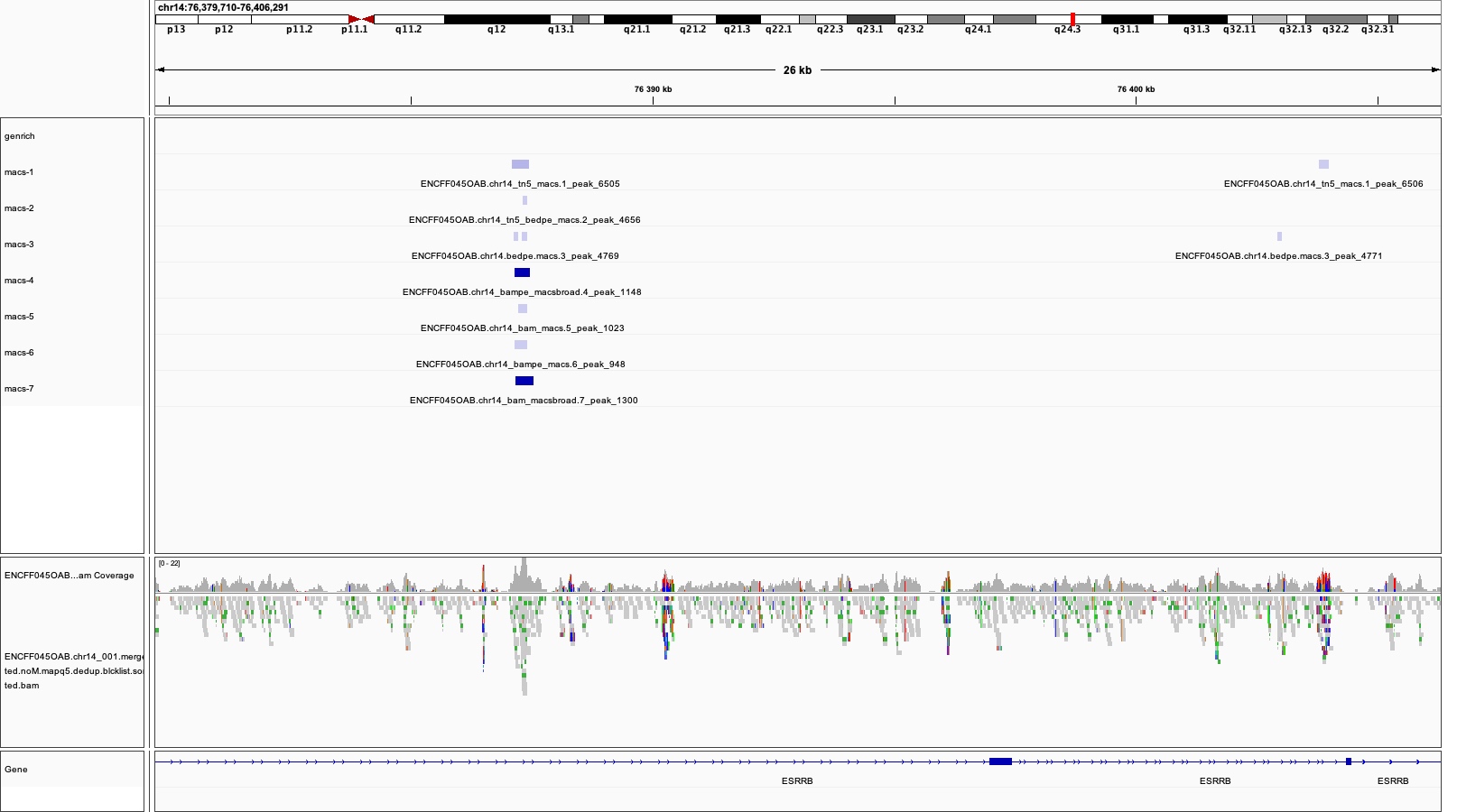

So which method to choose? You can test them all, for this tutorial we selected 4 and 5, which we found had most support in read coverage in regions we inspected yet still produced some spurious peaks. We’ll call the results broad and narrow, respectively. We use -g 107043718 for peak calling because this is the length of chr14, which is the only one included in the bam file. 那么选择哪种方法呢?您可以测试它们,在本教程中,我们选择了 4 和 5,我们发现在我们检查的区域的读取覆盖率方面支持最多,但仍会产生一些杂散峰。我们将结果分别称为“广泛”和“狭窄”。我们使用 '-g 107043718' 表示峰值调用,因为这是 chr14 的长度,这是 bam 文件中唯一包含的长度。
mkdir ../macs
cd ../macs

module load MACS/2.2.6

macs2 callpeak -t ../genrich/ENCFF045OAB.chr14.proc_rh.nsort.bam \
-n ENCFF045OAB.chr14.macs.broad --broad -f BAMPE \
-g 107043718 -q 0.1 --nomodel  --keep-dup all

macs2 callpeak -t ../genrich/ENCFF045OAB.chr14.proc_rh.nsort.bam \
-n ENCFF045OAB.chr14.macs.narrow -f BAM \
-g 107043718 -q 0.05 --nomodel --shift -75 --extsize 150 \
--call-summits --keep-dup all
How to shift reads in BED files
If you would like to test the effect of shifting reads, this how you do it on bed and bedpe files:
bedtools bamtobed -bedpe -i ENCFF045OAB.chr14.bam >ENCFF045OAB.chr14_pe.bed
bedtools bamtobed -i ENCFF045OAB.chr14.bam >ENCFF045OAB.chr14.bed

cat ENCFF045OAB.chr14.bed | awk -F $'\t' 'BEGIN {OFS = FS}{ if ($6 == "+") {$2 = $2 + 4} else if ($6 == "-") {$3 = $3 - 5} print $0}' >| ENCFF045OAB.chr14.proc.tn5.bed

cat ENCFF045OAB.chr14_pe.bed | awk -F $'\t' 'BEGIN {OFS = FS} {$2 = $2 + 4; $6 = $6 - 5; print $0}' >| ENCFF045OAB.chr14.proc.tn5.pe.bed
How many peaks were detected?
wc -l *Peak
 2011 ENCFF045OAB.chr14.macs.broad_peaks.broadPeak
 2428 ENCFF045OAB.chr14.macs.narrow_peaks.narrowPeak
Quite similar number of peaks for both methods, and double than what Genrich has detected. 两种方法的峰数非常相似,是Grich检测到的两倍。
ENCFF045OAB.chr14.macs.broad_peaks.broadPeak
head ENCFF045OAB.chr14.macs.broad_peaks.broadPeak
chr14   18674026        18674550        ENCFF045OAB.chr14.macs.broad_peak_1     21      .       3.15137 4.25082 2.12270
chr14   19096643        19097148        ENCFF045OAB.chr14.macs.broad_peak_2     31      .       3.61047 5.39085 3.19165
chr14   19098499        19098851        ENCFF045OAB.chr14.macs.broad_peak_3     16      .       2.95556 3.77788 1.68306
chr14   19105556        19105809        ENCFF045OAB.chr14.macs.broad_peak_4     27      .       3.42266 4.93515 2.76765
chr14   19161075        19162012        ENCFF045OAB.chr14.macs.broad_peak_5     24      .       3.29408 4.58492 2.42759
chr14   19172872        19173211        ENCFF045OAB.chr14.macs.broad_peak_6     22      .       3.19527 4.34825 2.20892
ENCFF045OAB.chr14.macs.narrow_peaks.narrowPeak
cd ..

module load BEDTools/2.25.0

bedtools intersect -a macs/ENCFF045OAB.chr14.macs.broad_peaks.broadPeak  -b genrich/ENCFF045OAB.chr14.genrich.narrowPeak  -f 0.50 -r >peaks_overlap.macs_broad.genrich.bed


bedtools intersect -a macs/ENCFF045OAB.chr14.macs.narrow_peaks.narrowPeak -b genrich/ENCFF045OAB.chr14.genrich.narrowPeak  -f 0.50 -r >peaks_overlap.macs_narrow.genrich.bed

wc -l *bed
   747 peaks_overlap.macs_broad.genrich.bed
 1613 peaks_overlap.macs_narrow.genrich.bed
Comparing results of MACS and Genrich
How many peaks actually overlap?
cd ..

module load BEDTools/2.25.0

bedtools intersect -a macs/ENCFF045OAB.chr14.macs.broad_peaks.broadPeak  -b genrich/ENCFF045OAB.chr14.genrich.narrowPeak  -f 0.50 -r >peaks_overlap.macs_broad.genrich.bed


bedtools intersect -a macs/ENCFF045OAB.chr14.macs.narrow_peaks.narrowPeak -b genrich/ENCFF045OAB.chr14.genrich.narrowPeak  -f 0.50 -r >peaks_overlap.macs_narrow.genrich.bed

wc -l *bed
   747 peaks_overlap.macs_broad.genrich.bed
 1613 peaks_overlap.macs_narrow.genrich.bed
Fraction of Reads in Peaks
Fraction of Reads in Peaks (FRiP) is one of key QC metrics of ATAC-seq data. According to ENCODE ATACseq data standards acceptable FRiP is >0.2. This value of course depends on the peak calling protocol, and as we have seen in the previous section, the results may vary …a lot. However, it is worth to keep in mind that any samples which show different value for this (and other) metric may be problematic in the analysis. 峰中读数分数(FRiP)是ATAC-seq数据的关键QC指标之一。根据ENCODE ATACseq数据标准可接受的FRiP为>0.2。这个值当然取决于峰值调用协议,正如我们在上一节中看到的,结果可能会有所不同......好多。但是,值得记住的是,任何显示此(和其他)指标不同值的样本在分析中都可能存在问题。
To calculate FRiP we need alignment file (bam) and peak file (narrowPeak, bed). 要计算FRiP,我们需要对齐文件(bam)和峰值文件(窄峰,床)。
Assuming we are in peaks:
mkdir frip
cd frip
We will use a tool called featureCounts from package Subread. This tool accepts genomic intervals in formats gtf/gff and saf. Let’s convert narrow/ broadPeak to saf:
awk -F $'\t' 'BEGIN {OFS = FS}{ $2=$2+1; peakid="macsBroadPeak_"++nr; print peakid,$1,$2,$3,"."}' ENCFF045OAB.chr14.macs.broad_peaks.broadPeak > ENCFF045OAB.chr14.macs.broad.saf
ENCFF045OAB.chr14.macs.broad.saf
macsBroadPeak_1 chr14   18674027        18674550        .
macsBroadPeak_2 chr14   19096644        19097148        .
macsBroadPeak_3 chr14   19098500        19098851        .
macsBroadPeak_4 chr14   19105557        19105809        .
macsBroadPeak_5 chr14   19161076        19162012        .
macsBroadPeak_6 chr14   19172873        19173211        .
We can now summarise reads:
ln -s ../genrich/ENCFF045OAB.chr14.proc_rh.nsort.bam

module load subread/2.0.0
featureCounts -p -F SAF -a ENCFF045OAB.chr14.macs.broad.saf --fracOverlap 0.2 -o ENCFF045OAB.peaks_macs_broad.counts ENCFF045OAB.chr14.proc_rh.nsort.bam
This command has produced reads summarised within each peak (which we won’t use) and a summary file ENCFF045OAB.peaks_macs_broad.counts.summary which contains values we are interested in:
Status  ENCFF045OAB.chr14.proc_rh.nsort.bam
Assigned        409482
Unassigned_Unmapped     0
Unassigned_Read_Type    0
Unassigned_Singleton    0
Unassigned_MappingQuality       0
Unassigned_Chimera      0
Unassigned_FragmentLength       0
Unassigned_Duplicate    0
Unassigned_MultiMapping 0
Unassigned_Secondary    0
Unassigned_NonSplit     0
Unassigned_NoFeatures   1247672
Unassigned_Overlapping_Length   6742
Unassigned_Ambiguity    1
409482/(1247672+6742+1+409482) = 0.246 (i.e. 24.6%)
featureCounts` reported in the output to the screen (STDOUT) that 24.6% reads fall within peaks, and this is FRiP for sample ENCFF045OAB.
Consensus Peaks
As our experiment has been replicated, we can select the peaks which were detected in both replicates. This removes non-reproducible peaks in regions of low coverage and other artifacts.由于我们的实验已经重复,我们可以选择在两个重复中检测到的峰。这样可以消除低覆盖率区域和其他伪影区域中不可重现的峰。
In this section we will work on peaks detected earlier using son-subset data.在本节中,我们将使用子集数据处理之前检测到的峰。
First we link necessary files:首先,我们链接必要的文件:
mkdir consensus
cd consensus

ln -s ../../../results/peaks/ENCFF045OAB.macs.broad_peaks.broadPeak
ln -s ../../../results/peaks/ENCFF363HBZ.macs.broad_peaks.broadPeak
ln -s ../../../results/peaks/ENCFF398QLV.macs.broad_peaks.broadPeak
ln -s ../../../results/peaks/ENCFF828ZPN.macs.broad_peaks.broadPeak
To recap, ENCFF398QLV and ENCFF363HBZ are untreated and ENCFF045OAB and ENCFF828ZPN are stimulated NK cells.
Let’s select peaks which overlap at their 50% length in both replicates (assumind we are in consensus):
module load BEDTools/2.25.0

bedtools intersect -a ENCFF398QLV.macs.broad_peaks.broadPeak -b ENCFF363HBZ.macs.broad_peaks.broadPeak  -f 0.50 -r >nk_peaks.bed
bedtools intersect -a ENCFF045OAB.macs.broad_peaks.broadPeak -b ENCFF828ZPN.macs.broad_peaks.broadPeak  -f 0.50 -r >nk_stim_peaks.bed
How many peaks?
wc -l *Peak
   51425 ENCFF045OAB.macs.broad_peaks.broadPeak
   54258 ENCFF363HBZ.macs.broad_peaks.broadPeak
   54691 ENCFF398QLV.macs.broad_peaks.broadPeak
   72067 ENCFF828ZPN.macs.broad_peaks.broadPeak
How many overlap?
wc -l *bed
  47156 nk_peaks.bed
  36606 nk_stim_peaks.bed
Merged Peaks
We can now merge the consensus peaks into peak sets used for downstream analyses.
bedops -m nk_peaks.bed nk_stim_peaks.bed > nk_merged_peaks.bed
The format of nk_merged_peaks.bed is very simple, 3-field BED file. Let’s add peaks ids and convert it to saf:
awk -F $'\t' 'BEGIN {OFS = FS}{ $2=$2+1; peakid="nk_merged_macsBroadPeak_"++nr;  print peakid,$1,$2,$3,"."}' nk_merged_peaks.bed > nk_merged_peaks.saf

awk -F $'\t' 'BEGIN {OFS = FS}{ $2=$2+1; peakid="nk_merged_macsBroadPeak_"++nr;  print $1,$2,$3,peakid,"0","."}' nk_merged_peaks.bed > nk_merged_peaksid.bed
These files can now be used in peak annotation and in comparative analyses, for example differential accessibility analysis.
We can now follow with downstream analyses: Peak Annotation, Differential Accessibility and TF footprinting.
Peak Annotation
Learning outcomes
Using ChIPseeker package
to profile ATAC-seq signal by genomics location and by proximity to TSS regions
to annotate peaks with the nearest gene
to run and compare functional enrichment
Introduction
In this tutorial we use an R / Bioconductor package ChIPseeker, to have a look at the ATAC / ChIP profiles, annotate peaks and visualise annotations. We will also perform functional annotation of peaks using clusterProfiler.
The tutorial is based on the ChIPseeker package tutorial so feel free to have this open alongside to read and experiment more.
Data & Methods
We will build upon the main labs:
ATAC-seq: all detected peaks (merged consensus peaks);
ATAC-seq: differentially accessible peaks;
Setting-up
You can continue working in the analysis/peaks/consensus directory.
We need access to file nk_merged_peaksid.bed and annotation libraries, whcih are preinstalled. We access them via:
module load R_packages/4.1.1
We activate R console upon typing R in the terminal.
We begin by loading necessary libraries:
library(ChIPseeker)
library(TxDb.Hsapiens.UCSC.hg38.knownGene)

library(GenomicAlignments)
library(GenomicFeatures)

library(clusterProfiler)
library(biomaRt)
library(org.Hs.eg.db)
library(ReactomePA)

txdb <- TxDb.Hsapiens.UCSC.hg38.knownGene
Peaks Coverage Plot
After peak calling one may want to visualise distribution of peaks locations over the whole genome. Function covplot calculates coverage of peaks regions over chromosomes. 在峰调用之后,人们可能希望可视化整个基因组中峰位置的分布。函数covplot计算染色体上峰区域的覆盖率。
Let’s load in the data (peaks called on nun subset data) and transform the data frame to GenomicRanges object (GRanges):让我们加载数据(在 nun 子集数据上调用的峰值)并将数据框转换为 GenomicRange 对象 (GRanges):
pth2peaks_bed="nk_merged_peaksid.bed"

peaks.bed=read.table(pth2peaks_bed, sep="\t", header=FALSE, blank.lines.skip=TRUE)
rownames(peaks.bed)=peaks.bed[,4]

peaks.gr <- GRanges(seqnames=peaks.bed[,1], ranges=IRanges(peaks.bed[,2], peaks.bed[,3]), strand="*", mcols=data.frame(peakID=peaks.bed[,4]))
If you are not familiar with GRanges objects, this is how the structure is:
> peaks.gr
GRanges object with 55108 ranges and 1 metadata column:
          seqnames              ranges strand |           mcols.peakID
             <Rle>           <IRanges>  <Rle> |            <character>
      [1]     chr1         10004-10442      * | nk_merged_macsBroadP..
      [2]     chr1         28945-29419      * | nk_merged_macsBroadP..
      [3]     chr1       180755-181858      * | nk_merged_macsBroadP..
      [4]     chr1       191246-191984      * | nk_merged_macsBroadP..
      [5]     chr1       778381-779290      * | nk_merged_macsBroadP..
      ...      ...                 ...    ... .                    ...
  [55104]     chrX 155880949-155881831      * | nk_merged_macsBroadP..
  [55105]     chrX 155997337-155997938      * | nk_merged_macsBroadP..
  [55106]     chrX 156016628-156016865      * | nk_merged_macsBroadP..
  [55107]     chrX 156025099-156025486      * | nk_merged_macsBroadP..
  [55108]     chrX 156030206-156030747      * | nk_merged_macsBroadP..
  -------
  seqinfo: 82 sequences from an unspecified genome; no seqlengths
To inspect peak coverage along the chromosomes:
covplot(peaks.gr, chrs=c("chr14", "chr15"))

#to save the image to file
pdf("PeakCoverage.pdf")
covplot(peaks.gr, chrs=c("chr14", "chr15"))
dev.off()

Peak Annotation
To annotate peaks with closest genomic features:
bed.annot = annotatePeak(peaks.gr, tssRegion=c(-3000, 3000),TxDb=txdb, annoDb="org.Hs.eg.db")
Let’s inspect the results:
> bed.annot
Annotated peaks generated by ChIPseeker
54970/55108  peaks were annotated
Genomic Annotation Summary:
              Feature   Frequency
9    Promoter (<=1kb) 32.22484992
10   Promoter (1-2kb)  3.95488448
11   Promoter (2-3kb)  3.41095143
4              5' UTR  0.34018556
3              3' UTR  2.07931599
1            1st Exon  1.87011097
7          Other Exon  2.72330362
2          1st Intron 11.74458796
8        Other Intron 21.09150446
6  Downstream (<=300)  0.09459705
5   Distal Intergenic 20.46570857
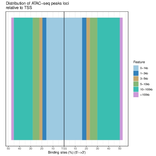
Over 30% of peaks localise to TSS, as expected in an ATAC-seq experiment.
Let’s see peak annotations:
annot_peaks=as.data.frame(bed.annot)
This is the resulting data frame:
 head(annot_peaks)
  seqnames  start    end width strand              mcols.peakID
1     chr1  10004  10442   439      * nk_merged_macsBroadPeak_1
2     chr1  28945  29419   475      * nk_merged_macsBroadPeak_2
3     chr1 180755 181858  1104      * nk_merged_macsBroadPeak_3
4     chr1 191246 191984   739      * nk_merged_macsBroadPeak_4
5     chr1 778381 779290   910      * nk_merged_macsBroadPeak_5
6     chr1 817270 817490   221      * nk_merged_macsBroadPeak_6
                                                   annotation geneChr geneStart
1                                            Promoter (1-2kb)       1     11869
2                                            Promoter (<=1kb)       1     14404
3                                            Promoter (<=1kb)       1    182696
4 Intron (ENST00000623083.4/ENST00000623083.4, intron 1 of 9)       1    187891
5                                            Promoter (<=1kb)       1    725885
6                                            Promoter (<=1kb)       1    817371
  geneEnd geneLength geneStrand    geneId      transcriptId distanceToTSS
1   14409       2541          1 100287102 ENST00000456328.2         -1427
2   29570      15167          2    653635 ENST00000488147.1           151
3  184174       1479          1 102725121 ENST00000624431.2          -838
4  187958         68          2 102466751 ENST00000612080.1         -3288
5  778626      52742          2 100288069 ENST00000506640.2             0
6  819837       2467          1    400728 ENST00000326734.2             0
          ENSEMBL       SYMBOL                                    GENENAME
1 ENSG00000223972      DDX11L1  DEAD/H-box helicase 11 like 1 (pseudogene)
2 ENSG00000227232       WASH7P           WASP family homolog 7, pseudogene
3 ENSG00000223972     DDX11L17 DEAD/H-box helicase 11 like 17 (pseudogene)
4 ENSG00000278267    MIR6859-1                             microRNA 6859-1
5            <NA> LOC100288069                uncharacterized LOC100288069
6 ENSG00000177757       FAM87B family with sequence similarity 87 member B
It can be saved to a file:
write.table(annot_peaks, "nk_merged_annotated.txt",
        append = FALSE,
        quote = FALSE,
        sep = "\t",
        row.names = FALSE,
        col.names = TRUE,
        fileEncoding = "")
We can also visualise the annotation summary:
pdf("AnnotVis.pdf")
upsetplot(bed.annot, vennpie=TRUE)
dev.off()

Distribution of loci with respect to TSS:
pdf("TSSdist.pdf")
plotDistToTSS(bed.annot, title="Distribution of ATAC-seq peaks loci\nrelative to TSS")
dev.off()
Functional Analysis
Having obtained annotations to nearest genes, we can perform functional enrichment analysis to identify predominant biological themes among these genes by incorporating knowledge provided by biological ontologies, e.g. GO (Gene Ontology, Ashburner et al. 2000) and Reactome (Croft et al. 2013).在获得最接近基因的注释后,我们可以进行功能富集分析,通过结合生物本体提供的知识来识别这些基因中的主要生物学主题,例如GO(Gene Ontology,Ashburner等人,2000)和Reactome(Croft等人,2013)。
In this tutorial we use the merged consensus peaks set. This analysis can also be performed on results of differential accessibility / occupancy.在本教程中,我们使用合并的共识峰集。该分析也可以对差异可达性/占用率的结果进行。
Let’s first annotate the peaks with Reactome.让我们首先用Reactome注释峰值。
Reactome pathway enrichment of genes defined as the nearest feature to the peaks: 被定义为最接近峰的特征的基因的反应组途径富集:
#finding enriched Reactome pathways using chromosome 1 and 2 genes as a background
pathway.reac <- enrichPathway(as.data.frame(annot_peaks)$geneId)

#previewing enriched Reactome pathways
head(pathway.reac)
This is the result (we skip column 8, as it is very broad - contains the gene IDs in set):
> colnames(as.data.frame(pathway.reac))
[1] "ID"          "Description" "GeneRatio"   "BgRatio"     "pvalue"
[6] "p.adjust"    "qvalue"      "geneID"      "Count"

> pathway.reac[1:10,c(1:7,9)]
                         ID                    Description GeneRatio   BgRatio
R-HSA-9012999 R-HSA-9012999               RHO GTPase cycle  407/8448 443/10856
R-HSA-9013149 R-HSA-9013149              RAC1 GTPase cycle  176/8448 185/10856
R-HSA-9013148 R-HSA-9013148             CDC42 GTPase cycle  151/8448 159/10856
R-HSA-4420097 R-HSA-4420097           VEGFA-VEGFR2 Pathway   97/8448  99/10856
R-HSA-194138   R-HSA-194138              Signaling by VEGF  105/8448 108/10856
R-HSA-9013404 R-HSA-9013404              RAC2 GTPase cycle   86/8448  88/10856
R-HSA-9013106 R-HSA-9013106              RHOC GTPase cycle   73/8448  74/10856
R-HSA-449147   R-HSA-449147      Signaling by Interleukins  402/8448 462/10856
R-HSA-8980692 R-HSA-8980692              RHOA GTPase cycle  137/8448 147/10856
R-HSA-5683057 R-HSA-5683057 MAPK family signaling cascades  287/8448 325/10856
                    pvalue     p.adjust       qvalue Count
R-HSA-9012999 7.645956e-16 1.161421e-12 8.893455e-13   407
R-HSA-9013149 4.636645e-11 3.521532e-08 2.696575e-08   176
R-HSA-9013148 1.771414e-09 8.969257e-07 6.868112e-07   151
R-HSA-4420097 6.278792e-09 2.384371e-06 1.825807e-06    97
R-HSA-194138  8.026320e-09 2.438396e-06 1.867176e-06   105
R-HSA-9013404 8.084405e-08 2.046702e-05 1.567240e-05    86
R-HSA-9013106 1.807641e-07 3.647964e-05 2.793389e-05    73
R-HSA-449147  1.921245e-07 3.647964e-05 2.793389e-05   402
R-HSA-8980692 3.786856e-07 6.391371e-05 4.894123e-05   137
R-HSA-5683057 5.815485e-07 8.479004e-05 6.492706e-05   287
We can see familar terms which can be connected to sample biology: Signaling by Interleukins, MAPK family signaling cascades.我们可以看到可以与样本生物学相关的熟悉术语:白细胞介素的信号传导,MAPK家族信号级联。
Let’s search for enriched GO terms:
pathway.GO <- enrichGO(as.data.frame(annot_peaks)$geneId, org.Hs.eg.db, ont = "MF")
These results look reasonable as well:
> pathway.GO[1:11,c(1,2,7)]
                   ID                                Description       qvalue
GO:0004674 GO:0004674   protein serine/threonine kinase activity 2.306759e-17
GO:0051020 GO:0051020                             GTPase binding 4.894211e-13
GO:0060090 GO:0060090                 molecular adaptor activity 5.215027e-13
GO:0030695 GO:0030695                  GTPase regulator activity 3.765106e-12
GO:0031267 GO:0031267                       small GTPase binding 8.221800e-12
GO:0030674 GO:0030674     protein-macromolecule adaptor activity 1.046226e-11
GO:0045296 GO:0045296                           cadherin binding 6.869553e-11
GO:0015631 GO:0015631                            tubulin binding 7.472641e-11
GO:0005085 GO:0005085 guanyl-nucleotide exchange factor activity 2.073955e-10
GO:0008017 GO:0008017                        microtubule binding 5.602393e-08
GO:0003712 GO:0003712         transcription coregulator activity 2.294003e-07
Differential Accessibility in ATAC-seq
Learning outcomes
to perform GC-aware normalisation of ATAC-seq data using EDASeq
to detect differentially accessible regions using edgeR
Introduction
In this tutorial we use an R / Bioconductor packages EDAseq and edgeR to perform normalisation and analysis of differential accessibility in ATAC-seq data.
Data & Methods
We will build upon the main lab ATACseq data analysis: - first we will summarise reads to detected peaks using subset data as an example to obtain a counts table; - we will use the counts table encompassing complete data for differential accessibility analysis;
Setting-up
We need access to file nk_merged_peaks.saf which we created in the ATACseq data analysis, part “Merged Peaks” and bam files with alignments.
Assuming we start at analysis:
mkdir counts_table
cd counts_table

ln -s ../peaks/consensus/nk_merged_peaks.saf
ln -s ../../data_proc/* .
Data Summarisation
We can now summarise the reads:
module load subread/2.0.0
featureCounts -p -F SAF -a nk_merged_peaks.saf --fracOverlap 0.2 -o nk_merged_peaks_macs_broad.counts ENCFF363HBZ.chr14.proc.bam ENCFF398QLV.chr14.proc.bam ENCFF828ZPN.chr14.proc.bam ENCFF045OAB.chr14.proc.bam
Let’s take a look inside the counts table using head nk_merged_peaks_macs_broad.counts.
# Program:featureCounts v2.0.0; Command:"featureCounts" "-p" "-F" "SAF" "-a" "nk_merged_peaks.saf" "--fracOverlap" "0.2" "-o" "nk_merged_peaks_macs_broad.counts" "ENCFF363HBZ.chr14.proc.bam" "ENCFF398QLV.chr14.proc.bam" "ENCFF828ZPN.chr14.proc.bam" "ENCFF045OAB.chr14.proc.bam"
Geneid  Chr     Start   End     Strand  Length  ENCFF363HBZ.chr14.proc.bam      ENCFF398QLV.chr14.proc.bam      ENCFF828ZPN.chr14.proc.bam      ENCFF045OAB.chr14.proc.bam
nk_merged_macsBroadPeak_1       chr1    10004   10442   .       439     5       10      15      20
nk_merged_macsBroadPeak_2       chr1    28945   29419   .       475     9       7       4       2
nk_merged_macsBroadPeak_3       chr1    180755  181858  .       1104    7       8       5       2
nk_merged_macsBroadPeak_4       chr1    191246  191984  .       739     0       3       1       0
nk_merged_macsBroadPeak_5       chr1    778381  779290  .       910     78      88      34      30
nk_merged_macsBroadPeak_6       chr1    817270  817490  .       221     0       0       0       0
nk_merged_macsBroadPeak_7       chr1    826976  827974  .       999     63      40      28      23
nk_merged_macsBroadPeak_8       chr1    838077  838576  .       500     0       1       0       0
We should remove the first line, as it can interfere with the way R reads in data:
awk '(NR>1)' nk_merged_peaks_macs_broad.counts > nk_merged_peaks_macs_broad.counts.tsv
Differential Accessibility
We activate R console upon typing R in the terminal.
We begin by loading necessary libraries:
library(edgeR)
library(EDASeq)

library(GenomicAlignments)
library(GenomicFeatures)

library(TxDb.Hsapiens.UCSC.hg38.knownGene)
library(wesanderson)

library(Hmisc)
library(dplyr)

txdb = TxDb.Hsapiens.UCSC.hg38.knownGene

ff = FaFile("/proj/epi2022/atacseq_proc/hg38ucsc/hg38.fa")


# We can read in the data, format it and define experimental groups:
cnt_table = read.table("../counts/nk_merged.macs_broad.counts", sep="\t", header=TRUE, blank.lines.skip=TRUE)
rownames(cnt_table)=cnt_table$Geneid

groups = factor(c(rep("NK",2),rep("NKstim",2)))

#this data frame contains only read counts to peaks on assembled chromosomes
reads.peak = cnt_table[,c(7:10)]


# We now prepare data with GC content of the peak regions for GC-aware normalisation.
gr = GRanges(seqnames=cnt_table$Chr, ranges=IRanges(cnt_table$Start, cnt_table$End), strand="*", mcols=data.frame(peakID=cnt_table$Geneid))

peakSeqs = getSeq(x=ff, gr)

gcContentPeaks = letterFrequency(peakSeqs, "GC",as.prob=TRUE)[,1]

#divide into 20 bins by GC content
gcGroups = Hmisc::cut2(gcContentPeaks, g=20)
mcols(gr)$gc = gcContentPeaks
Figure below shows that the accessibility measure of a particular genomic region is associated with its GC content. However, the slope and shape of the curves may differ between samples, which indicates that GC content effects are sample–specific and can therefore bias between–sample comparisons. 下图显示,特定基因组区域的可及性测量与其GC含量相关。然而,曲线的斜率和形状可能因样品而异,这表明GC含量效应是特定于样品的,因此可能会在样品比较之间产生偏差。
To visualise GC bias in peaks:
lowListGC = list()
for(kk in 1:ncol(reads.peak)){
  set.seed(kk)
  lowListGC[[kk]] = lowess(x=gcContentPeaks, y=log1p(reads.peak[,kk]), f=1/10)
}

names(lowListGC)=colnames(reads.peak)

dfList = list()
for(ss in 1:length(lowListGC)){
  oox = order(lowListGC[[ss]]$x)
  dfList[[ss]] = data.frame(x=lowListGC[[ss]]$x[oox], y=lowListGC[[ss]]$y[oox], sample=names(lowListGC)[[ss]])
}
dfAll = do.call(rbind, dfList)
dfAll$sample = factor(dfAll$sample)

p1.1 = ggplot(dfAll, aes(x=x, y=y, group=sample, color=sample)) +
  geom_line(size = 1) +
  xlab("GC-content") +
  ylab("log(count + 1)") +
  theme_classic()

pdf("GCcontent_peaks.pdf")
## plot just the average GC content
p1.1
dev.off()
 We can see that GC content has an effect on counts within the peaks.
We have seen from analyses presented on lecture slides (https://www.biorxiv.org/content/10.1101/2021.01.26.428252v2) that full quantile normalisation (FQ-FQ) implemented in package EDASeq is one of the methods which can mitigate the GC bias in detection of DA regions.
We’ll detect differentially accessible regions using edgeR. We will input the normalised GC content as offset to edgeR. 我们现在使用 edgeR 的统计框架。我们不像往常一样执行内部归一化 (TMM),而是提供由 EDASeq 计算的偏移量。
To calculate the offsets, which correct for library size as well as GC content (full quantile normalisation in both cases): 要计算偏移量,以校正文库大小和GC含量(两种情况下均为完全分位数归一化):
reads.peak=as.matrix(reads.peak)

dataOffset = withinLaneNormalization(reads.peak,y=gcContentPeaks,num.bins=20,which="full",offset=TRUE)
dataOffset = betweenLaneNormalization(reads.peak,which="full",offset=TRUE)
We now use the statistical framework of edgeR. We do not perform the internal normalisation (TMM) as usually, and instead we provide the offsets calculated by EDASeq. 我们现在使用 edgeR 的统计框架。我们不像往常一样执行内部归一化 (TMM),而是提供由 EDASeq 计算的偏移量。
design = model.matrix(~groups)

d = DGEList(counts=reads.peak, group=groups)

keep = filterByExpr(d)

> summary(keep)
        Mode   FALSE    TRUE
logical      21   54743


d=d[keep,,keep.lib.sizes=FALSE]

d$offset = -dataOffset[keep,]
d.eda = estimateGLMCommonDisp(d, design = design)
d.eda = estimateGLMCommonDisp(d, design = design)
fit = glmFit(d.eda, design = design)
lrt.EDASeq = glmLRT(fit, coef = 2)

DA_res=as.data.frame(topTags(lrt.EDASeq, nrow(lrt.EDASeq$table)))
The top DA peaks in stimulated vs non-stimulated NK cells:
> head(DA_res)

                                 logFC   logCPM       LR PValue FDR
nk_merged_macsBroadPeak_29593 7.743577 4.014714 1648.016      0   0
nk_merged_macsBroadPeak_9796  6.501470 4.527986 2801.485      0   0
nk_merged_macsBroadPeak_20351 6.490681 4.934009 3551.762      0   0
nk_merged_macsBroadPeak_12067 6.260759 4.441109 2593.194      0   0
nk_merged_macsBroadPeak_11203 6.165875 4.511952 2684.820      0   0
nk_merged_macsBroadPeak_53036 6.153595 4.023089 1922.240      0   0
Let’s add more peak information:
DA_res$Geneid = rownames(DA_res)
DA.res.coords = left_join(DA_res,cnt_table[1:4],by="Geneid")
We can check how well the GC correction worked:
gcGroups.sub=gcGroups[keep]
dfEdgeR = data.frame(logFC=log(2^lrt.EDASeq$table$logFC), gc=gcGroups.sub)

pedgeR = ggplot(dfEdgeR) +
  aes(x=gc, y=logFC, color=gc) +
  geom_violin() +
  geom_boxplot(width=0.1) +
  scale_color_manual(values=wesanderson::wes_palette("Zissou1", nlevels(gcGroups), "continuous")) +
  geom_abline(intercept = 0, slope = 0, col="black", lty=2) +
  ylim(c(-1,1)) +
  ggtitle("log2FCs in bins by GC content") +
  xlab("GC-content bin") +
  theme_bw()+
  theme(aspect.ratio = 1)+
  theme(axis.text.x = element_text(angle = 45, vjust = .5),
        legend.position = "none",
        axis.title = element_text(size=16))

ggsave(filename="log2FC_vs_GCcontent.pdf",plot=pedgeR ,path=".",device="pdf")

It seems that FQ-FQ normalisation did not completely remove the effect of GC content on log2FC in thie dataset. However, these effects are somewhat mitigated, you can compare this plot to one obtained by using the standard TMM normalisation.
The reason why the GC effects are not completely removed in this case may be that the DA analysis is not performed on properly replicated data; we should have at least 3 replicates per condition, and we only have two.
Transcription Factor Footprinting
Learning outcomes
detect transcription factor binding signatures in ATAC-seq data

Introduction
While ATAC-seq can uncover accessible regions where transcription factors (TFs) might bind, reliable identification of specific TF binding sites (TFBS) still relies on chromatin immunoprecipitation methods such as ChIP-seq. ChIP-seq methods require high input cell numbers, are limited to one TF per assay, and are further restricted to TFs for which antibodies are available. Therefore, it remains costly, or even impossible, to study the binding of multiple TFs in one experiment. 虽然 ATAC-seq 可以发现转录因子 (TF) 可能结合的可接近区域,但特定 TF 结合位点 (TFBS) 的可靠识别仍然依赖于染色质免疫沉淀方法,例如 ChIP-seq。 ChIP-seq 方法需要高输入细胞数,每次检测仅限于一个 TF,并且进一步仅限于可使用抗体的 TF。因此,在一项实验中研究多个转录因子的结合仍然是昂贵的,甚至是不可能的。
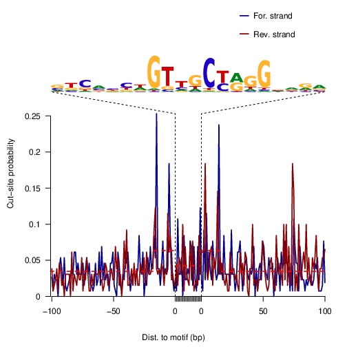
Similarly to nucleosomes, bound TFs hinder cleavage of DNA, resulting in footprints: defined regions of decreased signal strength within larger regions of high signal (Figure 1.).与核小体类似,结合的 TF 会阻碍 DNA 的裂解,从而产生足迹:在较大的高信号区域内确定信号强度降低的区域(图 1)。
Despite its compelling potential, a number of issues have rendered footprinting of ATAC-seq data cumbersome. It has been described that enzymes used in chromatin accessibility assays (e.g., DNase-I, Tn5) are biased towards certain sequence compositions. If unaccounted for, this impairs the discovery of true TF footprints.尽管其潜力巨大,但一些问题使得 ATAC-seq 数据的足迹变得很麻烦。据描述,染色质可及性测定中使用的酶(例如 DNase-I、Tn5)偏向于某些序列组成。如果下落不明,就会影响真正的 TF 足迹的发现。
In this tutorial we use an R / Bioconductor packages ATACseqQC and MotifDb to detect TF binding signatures in ATAC-seq data. Please note this tutorial is merely an early attempt to determine whether TF bindng sites can be identified in ATAC-seq data, and not a statistical framework for TF footrpinting. It can be used as a QC step to detect expected TF sites in the data rather than for discovery of novel binding patterns.在本教程中,我们使用 R / Bioconductor 包 ATACseqQC 和 MotifDb 来检测 ATAC-seq 数据中的 TF 结合特征。请注意,本教程只是确定是否可以在 ATAC-seq 数据中识别 TF 结合位点的早期尝试,而不是 TF 足迹分析的统计框架。它可以用作 QC 步骤来检测数据中预期的 TF 位点,而不是用于发现新的结合模式。
Data & Methods
We will build upon the lab ATACseq specifc QC and use the same data as for other ATAC-seq labs.我们将以实验室ATACseq特定的QC为基础,并使用与其他ATAC-seq实验室相同的数据。
Setting-up
We need access to bam file with shifted alignments shifted.bam which we created in the ATACseq specifc QC. This file contains alignments shifted +4 bps on the + strand and -5 bps on the - strand, to account for Tn5 transposition.我们需要访问我们在 ATACseq 特定 QC 中创建的具有移位对齐方式的 bam 文件。该文件包含 + 链上移位 +4 bps 和 - 链上移位 -5 bps 的对齐,以考虑 Tn5 转置。
Assuming we start at analysis:
mkdir TF_footprnt
cd TF_footprnt

ln -s ../QC/splitBam/shifted.bam .
ln -s ../QC/splitBam/shifted.bam.bai .

module load R_packages/4.1.1
Please check first that file shifted.bam exists in this location: ls ../QC/splitBam/shifted.bam. If it does, the output of this command is the path; if it does not you get “file does not exist”. Depending on the directory structure, you may need to link the file like this:請先檢查文件shifted.bam是否存在於這個位置:ls▁../QC/splitBam/shifted.bam。如果存在,此命令的輸出是路徑;如果不存在,則會得到「file▁does▁not▁exist」。根據目錄結構,您可能需要像這樣鏈接文件:
ln -s ../../QC/splitBam/shifted.bam .
ln -s ../../QC/splitBam/shifted.bam.bai .
Detection of TF Binding Signatures
We begin by loading necessary libraries:
library(ATACseqQC)
library(MotifDb)

library(BSgenome.Hsapiens.UCSC.hg38)
genome <- Hsapiens
Let’s first check signatures for a general TF CTCF. This is its motif as position weight matrix (PWM):
CTCF <- query(MotifDb, c("CTCF"))
CTCF <- as.list(CTCF)
print(CTCF[[1]], digits=2)
We now summarise the signal in the vicinity of CTCF motifs (100 bps up- and down-stream):
ctcf <- factorFootprints(shifted.bamFile, pfm=CTCF[[1]],
                         genome=genome,
                         min.score="90%", seqlev=seqlev,
                         upstream=100, downstream=100)
This function outputs signal mean values of coverage for positive strand and negative strand in feature regions, and other information which you can inspect using str(ctcf):此函数输出特征区域中正链和负链覆盖率的信号平均值,以及您可以使用str(ctcf)检查的其他信息: - spearman.correlation spearman correlations of cleavage counts in the highest 10-nucleotide-window斯皮尔曼相关性 最高10核苷酸窗口中切割计数的斯皮尔曼相关性 - bindingSites - GRanges object with detected bindng sites绑定站点 - 具有检测到的绑定站点的 GRanges 对象 - Profile.segmentation配置文件.分段
Let’s inspect the statistics ctcf$spearman.correlation:让我们检查一下统计数据ctcf$spearman.correlation:
> ctcf$spearman.correlation
$`+`

        Spearman's rank correlation rho

data:  predictedBindingSiteScore and highest.sig.windows
S = 3761558200, p-value < 2.2e-16
alternative hypothesis: true rho is not equal to 0
sample estimates:
      rho
0.2653951


$`-`

        Spearman's rank correlation rho

data:  predictedBindingSiteScore and highest.sig.windows
S = 3801340300, p-value < 2.2e-16
alternative hypothesis: true rho is not equal to 0
sample estimates:
      rho
0.2576259
The plot produced by this function is of signal mean values of coverage for positive strand and negative strand in feature regions.
pdf("ctcf_footprnt.pdf")
sigs <- factorFootprints(shifted.bamFile, pfm=CTCF[[1]],
                         genome=genome,
                         min.score="90%", seqlev=seqlev,
                         upstream=100, downstream=100)
dev.off()
We can generate similar plots for other TFs.
RFX5
RFX5 <- query(MotifDb, c("RFX5"))
RFX5 <- as.list(RFX5)


rfx5 <- factorFootprints(shifted.bamFile, pfm=RFX5[[1]],
                         genome=genome,
                         min.score="90%", seqlev=seqlev,
                         upstream=100, downstream=100)

 rfx5$spearman.correlation$`+`$estimate
 rfx5$spearman.correlation$`+`$p.value


pdf("rfx5_footprnt.pdf")
rfx5 <- factorFootprints(shifted.bamFile, pfm=RFX5[[1]],
                         genome=genome,
                         min.score="90%", seqlev=seqlev,
                         upstream=100, downstream=100)
dev.off()
STAT3
STAT3 <- query(MotifDb, c("STAT3"))
STAT3 <- as.list(STAT3)


stat3 <- factorFootprints(shifted.bamFile, pfm=STAT3[[1]],
                                 genome=genome,
                                 min.score="90%", seqlev=seqlev,
                                 upstream=100, downstream=100)

stat3$spearman.correlation$`+`$estimate
stat3$spearman.correlation$`+`$p.value

stat3$Profile.segmentation

pdf("stat3_footprnt.pdf")
stat3 <- factorFootprints(shifted.bamFile, pfm=STAT3[[1]],
                                 genome=genome,
                                 min.score="90%", seqlev=seqlev,
                                 upstream=100, downstream=100)
dev.off()
Which factors show evidence of binding enrichment in this data set?
Figure 2. Examples of TF footprints.
| CTCF | RFX5 | STAT3 |
|---|---|---|
 |
 |
 |
image source: https://doi.org/10.1038/s41467-020-18035-1 (Figure 1.)